Gradients of Deep Neural Networks: Vanishing Gradients and Residual Connections

August 6 2017

How can gradients propagate through networks with hundreds of layers? Why are LSTMs better than basic recurrent neural nets at learning long-term dependencies? I'd like to gain a better understanding of these questions by investigating the gradients of deep neural nets. Specifically, I'll be looking at the vanishing gradient problem and at the role residual connections play to address this problem.

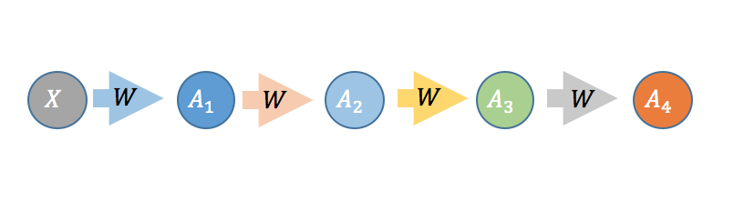
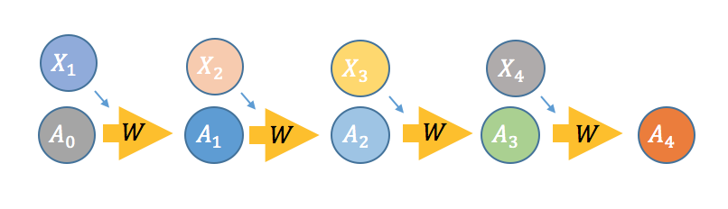
First, I'd like to note the similarities between deep neural nets (DNNs) and recurrent neural nets (RNNs). Comparing Fig 1 and Fig 2, we see that RNNs can be seen as DNNs but where the weights are the same at each layer and each layer gets a new input $X_t$ . In terms of backpropagation, adding layers to DNNs is similar to more timesteps for RNNs. Therefore, the issues related to gradients are similar in both DNNs and RNNs. For DNNs, its the weights that change at every layer. In RNNs, its the data that changes at every layer.

In Fig 1, the activations $A_t$ are computed as:

$\begin{align*} A_t &= f(W_t \cdot A_{t-1}) \\ \end{align*}$

where $f$ is a non-linear activation function (sigmoid, tanh, ReLu, Softplus, Maxout, Elu,...), $W_t$ is the $t^{th}$ layer weight matrix and $A_{t-1}$ are the activations of the previous layer. In the case of the RNN, $A_{t-1}$ is concatenated with the input $X_{t}$ . With the output $\hat{Y}$ and the target $Y$ , we will compute the objective $C(\hat{Y},Y)$ to minimize, where $C$ is some cost function (squared-error, cross-entropy,...). We'd like to now do gradient descent on the parameters of the model: $W_{new}=W_{old}-\alpha \frac{\partial C}{\partial W_{old}}$ , where $\alpha$ is the learning rate.

Vanishing and Exploding Gradients

For gradient descent, we need the partial derivatives of the weights with respect to (wrt) the cost function. We will first compute the gradients wrt the activations because obtaining the gradient wrt to the weights is simple once we have the gradients wrt the activations: $\frac{\partial C}{\partial W_t} = \frac{\partial C}{\partial A_t} \frac{\partial A_t}{\partial W_t}$ . Using the chain rule on a four layer net such as Fig 1, the gradients wrt some node $a$ in the third, second, and first layer are:

$\begin{align*} &\frac{\partial C}{\partial A^{(a)}_3} = \sum^{L_{4}}_i \frac{\partial C}{\partial A_4^{(i)}} \frac{\partial A_4^{(i)}}{\partial A^{(1)}_3} \\ &\frac{\partial C}{\partial A^{(a)}_2} = \sum^{L_{3}}_j \frac{\partial C}{\partial A^{(j)}_3} \frac{\partial A_3^{(j)}}{\partial A^{(a)}_2} = \sum^{L_{3}}_j \left( \sum^{L_{4}}_i \frac{\partial C}{\partial A_4^{(i)}} \frac{\partial A_4^{(i)}}{\partial A_3^{(j)}} \right) \frac{\partial A_3^{(j)}}{\partial A^{(a)}_2} \\ &\frac{\partial C}{\partial A^{(a)}_1} = \sum^{L_{2}}_k \frac{\partial C}{\partial A^{(k)}_2} \frac{\partial A_2^{(k)}}{\partial A_1^{(a)}} = \sum^{L_{2}}_k \left( \sum^{L_{3}}_j \left( \sum^{L_{4}}_i \frac{\partial C}{\partial A_4^{(i)}} \frac{\partial A_4^{(i)}}{\partial A_3^{(j)}} \right) \frac{\partial A_3^{(j)}}{\partial A_2^{(k)}} \right) \frac{\partial A_2^{(k)}}{\partial A_1^{(a)}} \\ \end{align*}$

where the sums are over the nodes of the respective layer and I've replaced $\hat{Y}$ with $A_4$ and $\frac{\partial A_t}{\partial A_{t-1}}$ is given by:

$\begin{align*} \frac{\partial A_t}{\partial A_{t-1}} &= \frac{\partial f(W_t \cdot A_{t-1})}{\partial A_{t-1} } = f^\prime(W_t \cdot A_{t-1})W_t\\ \end{align*}$

where $f^\prime$ is the derivative of the activation function.

In words, the above equations tell us that the gradient of a node equals the sum over the nodes of the next layer where each node is contributing a product of 1) its gradient, 2) the weight connecting the nodes, and 3) the gradient of the activation. A problem arises when these products are greater than one: the gradient will tend to explode because we are taking the product of many numbers greater than zero. Conversely, if its less than one, the gradient will tend to vanish. The sigmoid activation function is especially prone to the vanishing gradient given that its maximum gradient is 1/4.

Residual Connections

Lets change the architecture slightly. Rather than the node activation being the output of each node, lets add the activation to the previous activation, such that:

$\begin{align*} A_t &= f(W_t \cdot A_{t-1}) + A_{t-1} \\ \end{align*}$

With this change, the gradient of each activation wrt the previous activation becomes:

$\begin{align*} \frac{\partial A_t}{\partial A_{t-1}} &= \frac{\partial f(W_t \cdot A_{t-1})+ A_{t-1}}{\partial A_{t-1} } = f^\prime(W_t \cdot A_{t-1})W_t + 1 = Z+1\\ \end{align*}$

where $Z =f^\prime(W_t \cdot A_{t-1})W_t$ . Now let's look at the product of these gradients:

$\begin{align*} (Z+1)^2 &= Z^2 +2Z +1 \\ (Z+1)^3 &= Z^3 +3Z^2 +3Z +1 \\ (Z+1)^4 &= Z^4 +4Z^3 + 6Z^2 + 4Z +1 \end{align*}$

We see that even if $Z<0$ , the gradient does not vanish, resulting in the gradient persisting through the many layers of deep nets or long time horizons in RNNs. If the exploding gradient is a problem, it can be addressed in other ways, but that won't be discussed here.

Now lets compare the regular neural net activations versus the residual connection net by visualizing the gradients of a simple example. I trained a 20 layer net, where each layer has 20 units, on a dataset of random inputs and outputs of 20 dimensions. The activation function is tanh. In Fig 3 and Fig 4, the top row shows the forward propagation activations and the bottom row shows the gradients at each node.

In this case, the gradients of the regular network vanish after a few layers and very little learning is accomplished. In contrast, the gradients of the residual connections propagate all the way to the input layer.

In practice, the full story is more complex than the simple illustration above. Given different activations (ReLus, Elus), normalization techniques (batch norm, weight norm, layer norm), optimizers (Adam), and architectures (DenseNets), the gradient may exhibit different tendencies. However, these illustrations highlight some of the issues that need to be addressed in deep nets.

ResNet, HighwayNet, LSTM, GRU

Residual connections are the main idea of the ResNet paper. Highway Networks employ a similar idea, but with an extra gate, so that the activation becomes:

$\begin{align*} A_t &= f(W_t \cdot A_{t-1}) \cdot B + A_{t-1} \cdot (1-B) \\ B_t &= \sigma (W_{t}^{(2)} \cdot A_{t-1}) \end{align*}$

where $\sigma$ is the sigmoid output and $W_{t}^{(2)}$ is another weight matrix. These types of connections allow the networks to accommodate hundreds of layers. Prior to these deep network architectures, these ideas had been applied in the RNN setting. The Gated Recurrent Unit (GRU) already used the same activation as the one above. The most famous RNN, Long Short-Term Memory (LSTM), was introduced in 1997 and it used (along with other gates) similar ideas to enable long-term time dependencies.
Ilya Sustkever remarks in his PhD thesis that 'one of the earlier uses of skip connections was in the Nonlinear AutoRegressive with eXogenous inputs method (NARX; Lin et al., 1996), where they improved the RNN's ability to infer finite state machines'. Thus we see that these residual connections have appeared in a number of works and are an important element for propagating gradients in deep neural networks.